Dave & Dimi's Webspace
Averages
We all know how to take an average don't we? We take some numbers, divide by how many there are and Bob's your uncle, the answer is in front of you.
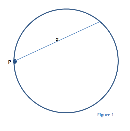 Take the following problem then. In Figure 1 there's a fixed point P on the edge of a circle:
What is the average distance (a) between P and the edge of the circle?
There are different types of average: geometric, harmonic, etc. but in this instance we refer to the most common one…
the arithmetic mean.
|
With certainty we could say that a is somewhere between zero and the diameter of the circle. That is to say,
… where r is the radius of the circle.
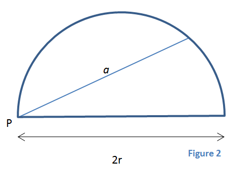 Also we could reason that drawing lines in the bottom half of the circle is a waste of time because for each line in the bottom half, a mirror image exists in the top half; so since we’re taking averages we may as well confine the argument to a semi-circle (see Figure 2) rather than a complete circle.
|
Dave's Reckoning
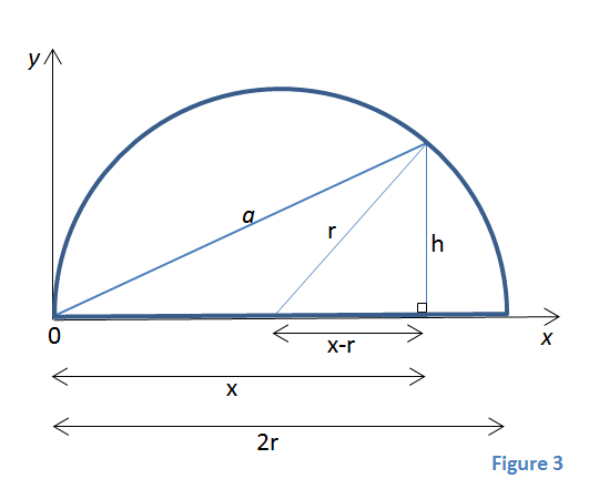 I did this by replacing the point P with the origin in a Cartesian coordinate system.
Then inserting a right-angled triangle that joins the mid-point of the diameter and the place where a intersects the semi-circle (see Figure 3).
|
Using Pythagoras' theorem, we can now construct two simultaneous equations,
|
|
r2 = (x - r)2 + h2
|
|
|
|
a2 = x2 + h2
|
|
Subtracting the bottom from the top yields,
|
|
r2 − a2 = (x − r)2 + h2 − (x2 + h2)
|
|
Funnily enough, all the r2, x2 and h2 terms cancel themselves out (isn't it great when that happens!?) and we end up with an expression for a,
From equation (1) we guessed that a had to be somewhere between 0 and 2r. Equation (2) does indeed confirm this because when x = 0 then a = 0.
Also, when x = 2r then a = 2r.
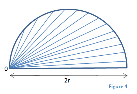 Just as there are infinite values of x, there are an infinite number of points on the semi-circle and of lines that can be drawn from 0 (Figure 4).
What we do next is to integrate equation (2) with respect to x, over all the infinite values that x could be (0 to 2r), then because we're taking an average, divide the result by that range. (It sounds a bit like cheating but it seems to be standard practice!)
|
|
a
|
=
|
1
|
∫
|
2r
|
√
|
2rx
|
dx
|
(3)
|
|
2r
|
0
|
The bar over the a in equation (3) is standard notation and indicates that we're taking a mean value.
Because we're integrating with respect to x, anything that isn't a function of x can be moved to the left of the integral sign,
|
|
a
|
=
|
√2r
|
∫
|
2r
|
√x
|
dx
|
(4)
|
|
2r
|
0
|
Regarding the integral we notice it contains a square root. Since √x is the same as x1/2 we use the normal integration procedure of adding 1 to the exponent then multiplying it by the reciprocal. So, adding 1 makes it x3/2 and the reciprocal of that exponent is 2/3,
|
|
a
|
=
|
√2r
|
[
|
2
|
x3/2
|
]
|
2r
|
(5)
|
|
2r
|
3
|
0
|
Substituting x with the high value 2r and low value 0,
|
|
a
|
=
|
√2r
|
(
|
(2r)3/2 − 03/2
|
)
|
(6)
|
|
3r
|
Tidying up,
And there we have it, an elegant mathematical proof that that the mean distance between a fixed point on a circle and its circumference is four thirds times the radius.
Dimi's Reckoning
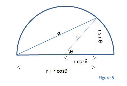 Dimi did this by using trigonometry.
He took the same semi-circle and introduced an angle that ranges from 0 to π (see Figure 5).
(Mathematical convention has it that the angle begins at zero on the x-axis then rotates anti-clockwise).
|
Again, applying Pythagoras' theorem, we get two simultaneous equations,
|
|
r2 = r2 cos2θ + r2 sin2θ
|
|
|
|
a2 = (r + r cos θ)2 + r2 sin2θ
|
|
Subtracting the bottom from the top yields,
|
|
r2 - a2 = r2 cos2θ + r2 sin2θ - ((r + r cosθ)2 + r2 sin2θ)
|
|
Once again a lot of cancelling out takes place and we're left with,
|
|
a = r
|
√
|
2
|
√
|
1 + cos θ
|
(8)
|
In equation (1) we figured that a had to be somewhere between 0 and 2r, so let's see...
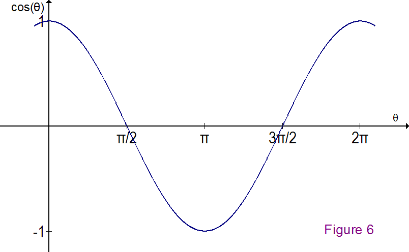 Using the cosine curve (Figure 6) we notice that if
θ = π
then
cos θ = -1
so equation (8) equals zero.
Furthermore, if
θ = 0
then
cos θ = 1
so equation (8) equals 2r.
|
Looking back at equation (1), this demonstrates that a is indeed between 0 and 2r.
What we do next is to integrate equation (8) with respect to θ, over all the range of values that θ could be (0 to π), then because we're taking an average, divide the result by that range (standard practice, I promise).
|
|
a
|
=
|
1
|
∫
|
π
|
r √
|
2
|
√
|
1 + cos θ
|
dθ
|
(9)
|
|
π
|
0
|
It so happens that,
1 + cos θ = 2 cos2(θ/2)
which is quite handy because taking integrals involving square roots is sometimes a messy job,
|
|
a
|
=
|
1
|
∫
|
π
|
r √
|
2
|
√
|
2 cos2 θ/2
|
dθ
|
(10)
|
|
π
|
0
|
Moving functions not related to θ to the left of the integral sign (because we're integrating with respect to θ only) and tidying up,
|
|
a
|
=
|
2r
|
∫
|
π
|
cos
|
θ/2
|
dθ
|
(11)
|
|
π
|
0
|
After integrating,
|
|
a
|
=
|
2r
|
[
|
2
|
sin θ/2
|
]
|
π
|
(12)
|
|
π
|
0
|
Substituting θ with the high value π and low value 0,
|
|
a
|
=
|
2r
|
(
|
2 sin
|
π/2
|
−
|
2 sin
|
0/2
|
)
|
(13)
|
|
π
|
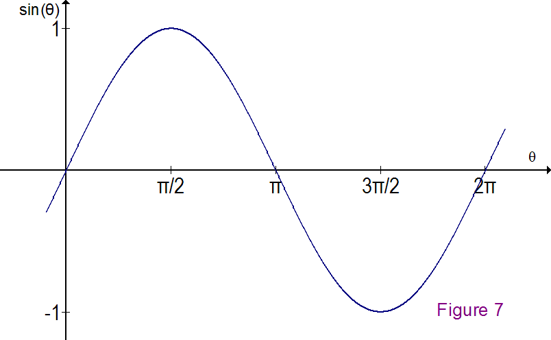
Referencing the sine curve (fig 7), we see that,
sin π/2 = 1
also that,
sin 0/2 = 0
Now substituting these values into equation (13)…
|
…leaves us with,
What went wrong?
Putting equations (7) and (14) side by side we're left with an obvious question: which one is correct? I mean, π equals 3.1415926535… and 3 equals, well, 3. But this is mathematics, surely there's no room for fuzzy estimates here!
The truth is that the problem was poorly stated. Means must be taken with respect to something. I used a horizontal axis beginning at zero and ending at 2r, Dimi used an angle starting at 0 and ending at π, it's not surprising we got different answers because we took our means with respect to different values!
Suppose we wanted to measure the average height of a person from birth to death. One statistician might do this by measuring their height every day. Another might do it by measuring their height every time they had a meal. It is highly likely that they would both get different results.
If nothing else this must be viewed as a cautionary tale with the message: Be careful when measuring averages.
Still not convinced?
I wasn't either… For years I suspected something fishy was going on. Infinities? Dividing them by ranges? Doing something “with respect” to something - uh? It's not exactly intuitively obvious is it!?
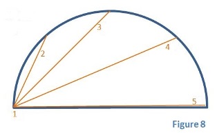 That's why I want to give you a solid, no-nonsense example here. One that doesn't faff around with concepts you might find, to say the least, dubious! It'll be messy but sometimes, you just gotta get your hands dirty ;-)
Rather than drawing an infinite number of lines, here we'll just take a small handful, say 5 of them, and space them out evenly over the semi circle.
Three of them (numbers 2, 3 and 4) are seen easily in Figure 8. If you look carefully you can see one running along the diameter (number 5). Also one of them (number 1) is zero-length so it's just there for the sake of neatness.
Using Dave's method to find the lengths of the lines (Figure 3, equation 2) we see:
| line length: |
1 |
2 |
3 |
4 |
5 |
| x = |
0 |
r/2 |
r |
3r/2 |
2r |
|
a = √
2rx
|
0 |
r |
r √ 2 |
r √ 3 |
2r |
Taking the average, (told you it was going to get messy!),
|
|
a
|
=
|
1
|
(
|
0 + r + r √2 + r √3 + 2r
|
)
|
=
|
r 1.22925…
|
|
|
5
|
Using Dimi's method (Figure 5, equation 8) we have:
| line length: |
1 |
2 |
3 |
4 |
5 |
| θ = |
0 |
π/4 |
π/2 |
3π/4 |
π |
|
a = r √2 √1 + cos θ
|
2r |
r √2 + √2
|
r √ 2
|
r √2 - √2
|
0 |
Taking the average,
|
|
a
|
=
|
1
|
(
|
2r + r √2 + √2
+ r √2 + r √2 - √2
+ 0
|
)
|
=
|
r 1.20546…
|
|
|
5
|
All is now revealed. Even though the lines were evenly spaced, three of them (1, 3 & 5) are of equal length, the crucial difference is found in lines 2 & 4.
Specifically,
and,
This is because I chopped up the x-axis into 5 equal sections and allowed vertical lines to intersect the semi-circle. Whereas Dimi, took an angle, divided it into 5 equal parts, let them radiate to the semi-circle and then dropped vertical lines from them.
In other words, I took my average with respect to the x-axis and he took his average with respect to an angle. Another mathematician could have used any other artibitary measure and their solution would be just as valid!
home